ResDAG
A modern, GPU-accelerated Reservoir Computing library for PyTorch. ResDAG brings the power of Echo State Networks (ESNs) and reservoir computing to PyTorch with a clean, modular API. Built for researchers and practitioners who need fast, flexible, and production-ready reservoir computing models.
- Lenguaje
- Python
- Estrellas
- 14
README

ResDAG
Reservoir computing for PyTorch.
Compose reservoir models as DAGs, train readouts with a single algebraic solve, run it all on the GPU.




ResDAG treats reservoir models — echo state networks and beyond — as ordinary PyTorch layers. Reservoirs, readouts, and transforms are nn.Modules wired together with a functional API; training a readout is one teacher-forced pass and one algebraic ridge solve, with no epochs. Models move with .to(device), serialize with state_dict(), and embed in larger PyTorch pipelines, optimizers included.
Track planned work and verification in the roadmap, with Pending, WIP and Done statuses.
Installation
pip install resdag            # core
pip install "resdag[hpo]"     # + Optuna hyperparameter optimization
Python ≥ 3.11, PyTorch ≥ 2.10.
Docs track
main. For unreleased changes, install from source:pip install "git+https://github.com/El3ssar/ResDAG". See the release history for packaged versions.
Try it
A reservoir forecaster on a toy signal, end to end:
import torch
import resdag as rd

t = torch.linspace(0, 60, 3000)
data = torch.sin(t).reshape(1, -1, 1)            # (batch, time, features)

warmup, train, target, f_warmup, val = rd.data.prepare_esn_data(
    data, warmup_steps=100, train_steps=2000, val_steps=300)

model = rd.models.classic_esn(reservoir_size=300, feedback_size=1, output_size=1)
rd.ESNTrainer(model).fit((warmup,), (train,), targets={"output": target})

prediction = model.forecast(f_warmup, horizon=300)   # autoregressive, (1, 300, 1)
The first forecast walkthrough does the same on the Lorenz attractor, with the math explained.
The end-to-end guide covers data preparation, fitting, evaluation, saving and reuse inside a larger PyTorch model. Run its small complete example with uv run python examples/15_end_to_end.py.
Choose and customize the memory
Use leaky ESNs, oscillators, Legendre delay memory, spiking reservoirs, or
wrapped PyTorch GRU/LSTM cells through the same composition API. Select recurrent
weights with recurrent_initializer=; names, parameter tuples, callables and
custom registration all work. Biases, reset states and gated recurrence have
separate hooks. Optional intrinsic plasticity and flow control calibrate a
standard ESN on training inputs before fitting its readout.
Start with recurrent weights, custom registration, the layer catalog, or calibration.
Compose, don't configure
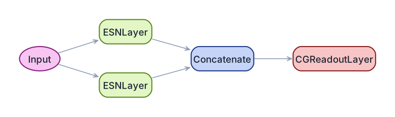
Architectures are DAGs you wire, not options you toggle. Two reservoirs on different timescales, read out together:
from resdag import CGReadoutLayer, Concatenate, ESNModel, reservoir_input
from resdag.layers import ESNLayer

inp    = reservoir_input(3)
fast   = ESNLayer(64, feedback_size=3, leak_rate=1.0, spectral_radius=0.9)(inp)
slow   = ESNLayer(64, feedback_size=3, leak_rate=0.2, spectral_radius=0.9)(inp)
merged = Concatenate()(fast, slow)
model  = ESNModel(inp, CGReadoutLayer(128, 3, name="output")(merged))
Branches, feature augmentations, and multiple readout heads compose the same way — one reservoir, squared-state augmentation, two heads:
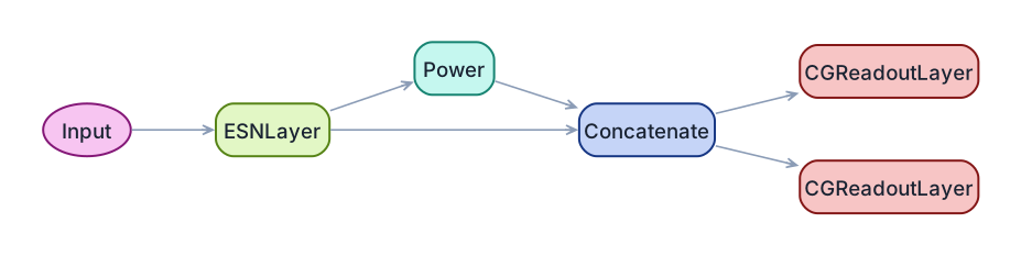
All heads fit in a single pass, in dependency order. The composition handbook covers the patterns.
Coming from scikit-learn?
The whole fit → predict loop fits in one object. ESN.fit(series) slices the warmup window, builds the one-step-ahead target, and runs the algebraic solve; forecast(horizon=...) re-synchronizes and rolls out — numpy in, numpy out:
import numpy as np
from resdag import ESN

series = np.cumsum(np.random.randn(2000, 3), axis=0)   # (time, features)

esn = ESN(reservoir_size=300, spectral_radius=0.9).fit(series)
prediction = esn.forecast(horizon=200)                 # (200, 3)
esn.model drops you back into the full composable graph whenever you outgrow the facade. The mental model maps fit/predict onto ResDAG's warmup + ESNTrainer.fit / forecast flow.
Train through it with SGD
A reservoir is an ordinary PyTorch layer, so it drops into a pipeline as a frozen feature extractor and you train any head with a normal optimizer loop. The reservoir has zero trainable parameters, so the optimizer only ever touches the head:
import torch
import torch.nn as nn
from resdag import ReservoirFeatureExtractor

net = nn.Sequential(
    ReservoirFeatureExtractor(500, feedback_size=3, spectral_radius=0.9, stateful=False),
    nn.Linear(500, 64), nn.Tanh(), nn.Linear(64, n_classes),
)
extractor, head = net[0], net[1:]
opt = torch.optim.Adam(head.parameters(), lr=1e-3)     # head only — reservoir is frozen

with torch.no_grad():                                  # frozen features: compute once
    extractor.on_epoch_start()
    feats = extractor(sequences)[:, -1]                # (batch, 500) last-step summary

for _ in range(300):
    loss = nn.functional.cross_entropy(head(feats), labels)
    opt.zero_grad(); loss.backward(); opt.step()
This is the pure-PyTorch path: gradient heads, full BPTT through the recurrence (trainable=True), and embedding frozen reservoirs in larger networks. Work · Train covers all three training paths; Work · Scale & deploy shows the frozen-backbone classifier inside a nn.Module pipeline.
For independent minibatches, stateful=False starts from zeros on each call.
The default carries state across calls for streaming. Frozen weights still
allow gradients to flow to an upstream neural encoder. Keep the complete
trained esn.model inside a larger nn.Module when you need its readout and
all DAG branches; reset its reservoirs between independent sequences.
Premade factories accept a readout name or class, plus separate solver options:
model = rd.classic_esn(
    reservoir_size=300, feedback_size=3, output_size=3,
    readout="svd", readout_alpha=1e-6,
    readout_kwargs={"trainable": True, "rcond": 1e-12},
)
This fits algebraically with ESNTrainer and lets an optimizer fine-tune the
same readout afterwards. Available names are ridge, cholesky, cg, svd,
pinv, incremental, rls, and fista. SVD and pseudoinverse fitting operate
directly on the design matrix without allocating a feature-by-feature Gram.
Documentation
| Start | Install, a first trained forecaster, the mental model |
| Build | Layers, readouts, architectures, topologies, initializers |
| Work | Training paths, forecasting with drivers, tuning, GPU |
| Theory | Every equation, stated against the code |
| Reference | The full public API |
Ecosystem
Built on pytorch_symbolic for graph composition. Pairs with TSDynamics, a companion library of dynamical systems — it generates the systems, ResDAG forecasts them.
Contributing
See CONTRIBUTING.md — releases are automated from conventional commits, and most component types are one registry decorator away.
License
MIT — © Daniel Estevez-Moya
Software

TSDynamics
TSDynamics: A Python package for defining and simulating continuous and discrete dynamical systems, including time-delay equations and maps. With a user-friendly interface for RHS definitions, it provides tools for numerical analysis and aims to integrate advanced time series analysis tools..
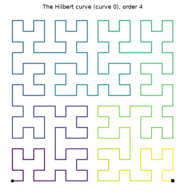
hilbertplot
The complete set of 40 two-dimensional Hilbert curves, and fast data plots on them.

lzcomplexity
lzcomplexity is a high-performance C++ library developed for complexity analysis using entropic magnitudes. The library provides efficient implementations for analyzing time series data, with applications in information theory, signal processing, and neuroscience.