hilbertplot

The complete set of 40 two-dimensional Hilbert curves — and a fast way to plot long 1-D data on any of them.

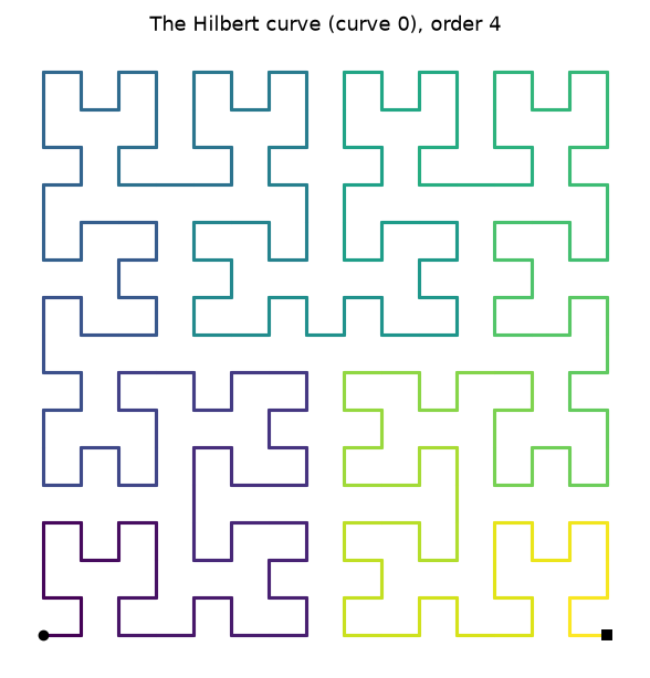
Most software knows one Hilbert curve. In fact there are forty distinct space-filling curves of Hilbert type in two dimensions (up to rotation, reflection and reversion), as proved by Estevez-Rams et al., "Hilbert curves in two dimensions", Rev. Cub. Fís. 34, 9 (2017). hilbertplot implements all forty with pure-numpy generation and uses them to lay long 1-D vectors onto 2-D images.

Install

pip install "hilbertplot[plot]"   # drop [plot] for a numpy-only core (no matplotlib)

Draw a curve

import hilbertplot

c = hilbertplot.curve(0)     # by index 0–39, by name ("Moore"), or by symbol
c.show(4)                    # draw order 4 in a window
pts = c.points(4)            # (256, 2) integer lattice points, in visit order

The forty curves come in named groups — hilbertplot.proper(), .improper(), .homogeneous(), .inhomogeneous(), .generalizing() — each of which prints as a table, and which compose:

import hilbertplot

print(hilbertplot.proper())                       # a table of the six proper curves
hilbertplot.catalog().closed().names              # ['Moore', 'Liu1', 'Improper1', 'Improper4']
hilbertplot.by_kernels(3, 5).gallery(order=3)     # draw a group as a grid of panels

In a Jupyter notebook a Curve renders itself — put hilbertplot.curve("Moore") in a cell and you get the picture, not a repr.

One cell at a time

points(order) builds all 4**order cells. When you only need where step i lands, encode answers in O(order) — so it works at orders no machine could materialise, and it does so for all forty curves, not just the classic one:

import hilbertplot

c = hilbertplot.curve(0)
c.encode(5, 2)                     # (0, 3) — the cell visited at step 5, order 2
c.decode(0, 3, 2)                  # 5      — and back again
c.encode(10**18, 40)               # (751054336, 346100736) — a 2**80-cell curve

Plot data

Walk a curve and drop data[i] on the i-th cell it visits: a locality-preserving 1-D → 2-D map where nearby values stay nearby.

import numpy as np, hilbertplot

plot = hilbertplot.hilbert_plot(0, np.arange(1, 257))
plot.show("viridis")          # a matplotlib colormap name, or a list of colours to blend

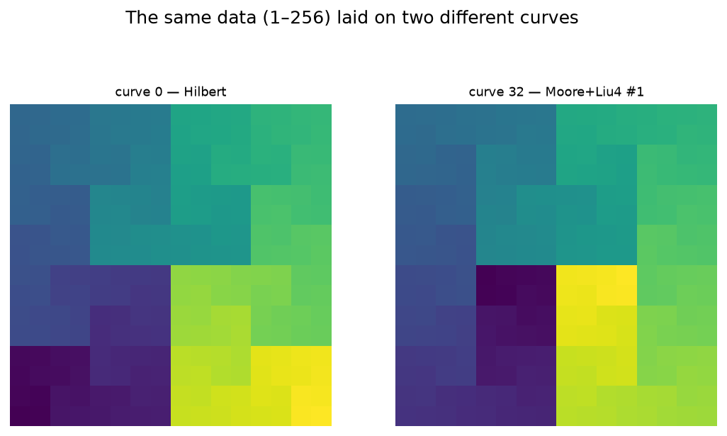
The same numbers on curve 0 and curve 32 — one reason to have all forty.

Seeing more than the data

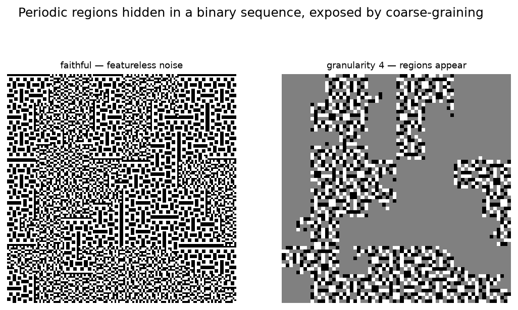
Coarse-grain it. plot.show(granularity=4) replaces each block of values by its mean. Below, a binary sequence interleaves stretches of two periodic patterns with identical density — invisible in the faithful plot, obvious once averaged.

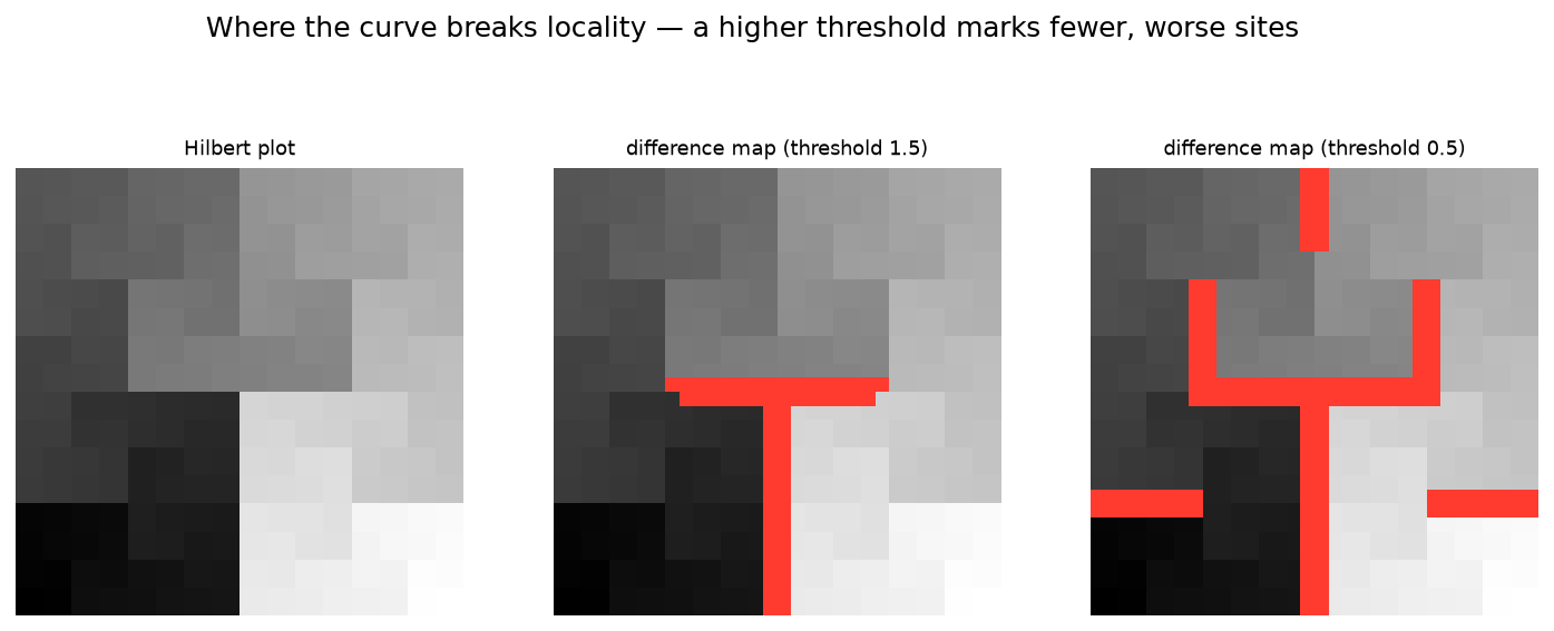
Find where locality breaks. plot.show(difference=True) marks the cells that are neighbours in the plane but far apart along the curve. A higher threshold keeps only the worst offenders.

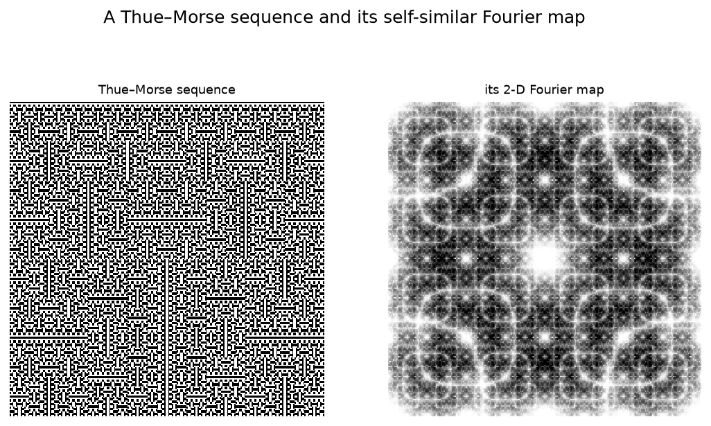
Transform it. plot.show(fourier=True) renders the 2-D Fourier map, exposing periodic and self-similar structure — here, a Thue–Morse sequence.

Also

• curve.unroll(img) — read a 2-D array back into 1-D, in curve order
• curve.grid(n) — the eight generalizing() curves tile any n×n square, not just 2ᵏ
• curve.label_map(order) — the grid of visit indices, as an image
• curve.difference_map(order) — where the curve breaks locality, as a field
• plot.draw(colorbar=True), or norm=LogNorm() for heavy-tailed data
• hilbertplot.is_space_filling / canonical_form — check a path yourself; the same tools the test suite uses to prove all forty curves are distinct Hamiltonian paths
• hilbertplot.clear_cache() / cache_info() — generated curves are memoised; this frees them
• hilbertplot.set_cell_limit(n) — raise the guard that refuses absurdly large orders

Every figure above is reproducible: python examples/readme_figures.py. More runnable demos are in examples/; the arbitrary-square classification and its impossibility proofs are in the repository's research/quasisquares/.

License

MIT © Daniel Estevez — LICENSE