TSDynamics
TSDynamics: A Python package for defining and simulating continuous and discrete dynamical systems, including time-delay equations and maps. With a user-friendly interface for RHS definitions, it provides tools for numerical analysis and aims to integrate advanced time series analysis tools..
- Language
- Python
- Stars
- 3
README
TSDynamics


Dynamical systems in Python: 177 built-in systems, a native Rust integration engine, and a chaos-analysis toolkit.
You write the math (one symbolic method); TSDynamics lowers it to a native Rust engine and handles integration, Lyapunov spectra, bifurcation diagrams, Poincaré sections, attractors & basins — and even the documentation page for your system.
A built-in Lorenz attractor — integrated, spun, and saved to a GIF (code below).
import tsdynamics as ts

lor = ts.systems.Lorenz(ic=[1.0, 1.0, 1.0])
traj = lor.run(final_time=100.0, dt=0.01)   # `run` is the one verb, every family
traj["x"]                                   # named component access

print(ts.analysis.lyapunov_spectrum(lor))   # an analysis is a free function
# LyapunovSpectrum  λ = [0.916, 0.0001893, -14.58]   chaotic · D_KY = 2.063   (Lorenz)
📖 Documentation: https://el3ssar.github.io/TSDynamics/
Define your own system
import tsdynamics as ts

class Rossler(ts.ContinuousSystem):
    variables = ("x", "y", "z")            # dim inferred = 3
    params = {"a": 0.2, "b": 0.2, "c": 5.7}
    _reference = "Rössler (1976), Phys. Lett. A 57, 397-398"

    def _equations(y, t, a, b, c):
        x, yv, z = y(0), y(1), y(2)
        return (-yv - z, x + a * yv, b + z * (x - c))
That's the whole ODE contract. The class auto-registers and works with analyses
that accept flows. For systems added to the built-in catalogue, the test suite
sweeps them and the docs build renders their equations and attractors. Delay
systems use y(0, t - tau); maps implement _step (the Jacobian is derived from
it); SDEs add a _diffusion term. Rossler().info prints everything the library
read back to you.
From equations to figures
There is one plotting verb, and it has one rule: ts.plot draws everything
you hand it on one figure and gives you back a Plot — a positional string
says how to draw, everything else says what to draw, and a Plot handed back in
is just another thing to draw. That last clause is why grids, movies and
escape-to-matplotlib need no extra API. The Plot is backend-neutral: tweak it
fluently, then save to matplotlib, plotly (interactive), three.js or JSON.
Bifurcation diagram of the logistic map, with the period-doubling onsets
marked — orbit_diagram is one call, and .bifurcation_points() finds the
cascade ($r_1 = 3$, $r_2 = 1 + \sqrt6 \approx 3.449$, …):
import numpy as np, tsdynamics as ts

orbit = ts.analysis.orbit_diagram(ts.systems.Logistic(), "r", np.linspace(2.8, 4.0, 2000))
pts = orbit.bifurcation_points()

p = ts.plot(orbit, color="k", markersize=0.2, alpha=0.5,   # tiny translucent dots
            xlabel="r", ylabel="x*", title="Logistic bifurcation")
for i, lbl in [(0, " r₁"), (1, " r₂"), (3, " r₄")]:        # mark the onsets
    p.vline(pts[i], label=lbl, color="red", linestyle="dashed")
p.save("bifurcation.png", size=(1600, 700))
A PDE, too — the Kuramoto–Sivashinsky equation is a built-in spatially extended system; its space–time field is auto-detected and drawn as a heatmap:
import tsdynamics as ts

ks = ts.systems.KuramotoSivashinsky(N=128, L=22.0)
traj = ks.run(final_time=200.0, dt=0.25)
ts.plot(traj).save("ks.png")              # 128-mode space–time field
Named plots, grids, primitives. Beyond the auto-detected default, a
positional string names a plot transform — 38 of them, from nullclines and
streamlines to ftle, cobweb, invariant_density and trace_determinant.
Each declares which primitives can draw it, so you pick the drawing without
touching a backend; and because a Plot is itself a legal subject, a grid of
different plots is the same call:
import numpy as np, tsdynamics as ts

vdp = ts.systems.VanDerPol(params={"mu": 1.0})
traj = vdp.run(final_time=30.0, dt=0.01, ic=[0.5, 0.0])

ts.plot(vdp, traj, "flow_speed", "nullclines")                   # overlay, order-free
ts.plot(ts.plot(traj), ts.plot(traj, "psd"), layout="row")       # a grid
ts.viz.draw({"x": np.arange(5.0), "y": np.arange(5.0) ** 2}, "line")   # bare arrays

@ts.viz.transforms.register(source="data", frame="time", kind="diagnostic_curve",
                            primitives=("line", "points"))
def speed(traj):
    """Instantaneous speed |dx/dt| along the orbit."""
    return {"x": traj.t[1:],
            "y": np.linalg.norm(np.diff(traj.y, axis=0), axis=1) / np.diff(traj.t)}

ts.plot(traj, "speed")   # ...now in the gallery, the matrix, and every plot door
A transform owns no new math — it adapts an estimator from tsdynamics.analysis.
The gallery is
generated from the registry, so every picture there is produced by the snippet
printed beside it.
The spinning attractor at the top is the same call, animated:
import tsdynamics as ts

traj = ts.systems.Lorenz().run(final_time=100.0, dt=0.01)
p = ts.plot(traj, animate=True)
p.style(axes=False).trail(None).camera(spin=0.4)      # full curve, no axes, rotate
p.animate(fps=30, duration=10, loop=True)
p.save("lorenz.gif")
A taste of the analysis layer
import numpy as np, tsdynamics as ts

# Poincaré section of the Rössler attractor (root-refined crossings)
section = ts.analysis.poincare_section(ts.systems.Rossler(), plane=("y", 0.0, "up"), crossings=500)

# Fixed points of the Hénon map, with stability — the repr IS the report
print(ts.analysis.fixed_points(ts.systems.Henon()))
# FixedPointSet  2 points · 0 stable, 2 unstable   (Henon)
#     [0] x* = [-1.1314 -0.3394]  unstable  |λ|max = 3.26
#     [1] x* = [0.6314 0.1894]  unstable  |λ|max = 1.924

# Maximal Lyapunov exponent — no Jacobian needed
ts.analysis.lyapunov_spectrum(ts.systems.Lorenz(), k=1, ic=[1, 1, 1])     # ≈ 0.90
Plus: attractors & basins of any flow or map, correlation/Rényi fractal dimensions, RQA (recurrence quantification), delay embedding (Takens, optimal τ, Cao/FNN), periodic orbits (shooting, Davidchack–Lai), numerical interval search for fixed points, GALI, the 0–1 chaos test & Hunt–Ott expansion entropy, and Lyapunov exponents from a bare time series (Kantz/Rosenstein).
Highlights
Four families, one interface — ODEs, DDEs, SDEs and discrete maps all answer the same
runverb and the same stepping protocol (reinit/step/state/time). Each analysis documents the families and inputs it supports;ts.analysis.find(system)lists compatible routines.A small surface —
tsdynamics.<TAB>is 11 names,lorenz.<TAB>is 20, and every analysis is a free function whose first argument is its subject (ts.analysis.lyapunov_spectrum(lorenz)). A name that moved raises an error printing its new address; that error is the migration guide.177 built-in systems with literature parameters (142 ODEs, 26 maps, 6 DDEs, 3 SDEs).
Native engine: equations lower to a Rust engine in-process and run on a built-in Cranelift JIT (or a bit-for-bit identical SSA-tape interpreter); ordinary parameters are runtime values, so changing them reuses the tape. Structural parameters and delay values require fresh lowering. The engine writes no compilation cache to disk.
For adaptive ODE solvers,
dtsamples,rtoldecides — the output grid and the accuracy knob are separate. The adaptive steppers use genuine dense output, so a coarsedtis cheap without being less accurate, andmax_step=is there when you need to bound the step explicitly. Defaults arertol=1e-9/atol=1e-12.Composition — a Poincaré section of a flow is a discrete map, so
ts.analysis.orbit_diagram(ros.poincare("y", 0.0), "c", values)draws the bifurcation diagram of a flow in one line.Backend-neutral plotting — one
Plotrenders to matplotlib, plotly (interactive + animated HTML), three.js, or JSON, with a fluent styling/theming vocabulary and registries for transforms, primitives, themes and renderers.
Install
pip install tsdynamics # or: uv add tsdynamics
A prebuilt abi3 wheel (manylinux / musllinux / macOS / Windows) bundles the
native Rust engine. No Rust toolchain and no C compiler needed to install or
run. Optional plotting extra: tsdynamics[plot,interactive] (matplotlib, plotly).
Development
git clone https://github.com/El3ssar/TSDynamics && cd TSDynamics
uv sync --group dev --group docs
make test                                # change-scoped fast tier (the loop)
make test-slow                           # change-scoped slow tier
make test-all                            # whole fast tier — pre-push sanity
TSD_DOCS_FIGURES=0 uv run mkdocs serve   # docs preview
The suite is registry-driven — every test is parametrized over all 177 systems —
so a plain pytest is thousands of items. make test runs only what your diff
touches, which is what CI does too.
Releases are automated: conventional-commit PR titles drive semantic-release on merge. See CONTRIBUTING.
License
MIT © Daniel Estevez
Software

ResDAG
A modern, GPU-accelerated Reservoir Computing library for PyTorch. ResDAG brings the power of Echo State Networks (ESNs) and reservoir computing to PyTorch with a clean, modular API. Built for researchers and practitioners who need fast, flexible, and production-ready reservoir computing models.
hilbertplot
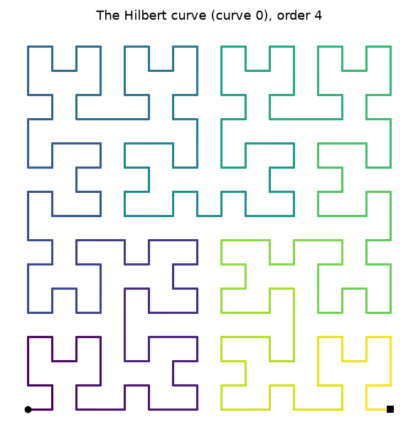
The complete set of 40 two-dimensional Hilbert curves, and fast data plots on them.

lzcomplexity
lzcomplexity is a high-performance C++ library developed for complexity analysis using entropic magnitudes. The library provides efficient implementations for analyzing time series data, with applications in information theory, signal processing, and neuroscience.